A Little Rusty? ML Refresher on Linear Regression
John Inacay, Mike Wang, and Wiley Wang (All authors contributed equally)
In the field of Machine Learning, many ML practitioners started out learning and understanding classical ML algorithms. However, lack of practice can dull your mastery of these algorithms. We would like to start a series of blogs to help refresh ML algorithms.
You may have learned linear regression in college. Now that several years have passed by, you vaguely remember what it is. Deep Learning is everywhere in the field when solving machine learning problems. In a traditional deep learning pipeline, we’re used to collecting large amounts of data and fitting them to a deep learning model, sometimes without fully understanding how the model works. It all feels magical when you see 97% accuracy out of the box making us in awe of modern machine learning. But in the back of your mind, have you ever wondered, was it necessary to learn the older traditional machine learning methods? The answer might feel like a distant “yes”. We’re starting a Refresher Series to help you remember traditional Machine Learning. In this blog post, we’ll cover the Linear Regression algorithm.
What Is Linear Regression?
Let’s start off with a definition of what linear regression is: a method of modeling a linear (technically, affine) correlation between an input vector to an output. We obtain data of some known inputs paired with some known outputs. We want to use these known inputs to create a model that can reproduce the output given the same inputs.
Basically:
y=ax+b, where y is the output and x is in the input vector
We’re finding the vectors a and b (the model) that minimizes the mean squared error (mse) between the calculated y and the actual output in the data. Note: mean square error optimization is not unique to linear regression (there is a non-linear least square problem formulation).
How Do We Use Linear Regression?
Linear regression is simply predicting a value given one or more input values. Basically, if we want to know a number, we might be able to estimate the true value with our model. However, the linear regression technique only works if there’s a linear relationship between the input and output.
While it’s one of the tools we have, it may or may not be the right tool for the task we have. Linear relationships are common in data, but real life data are much more complex than linear relationships. Here are some guidelines when it comes to linear regression:
- Start simple, use linear regression as a baseline algorithm.
- Large dimension data? You may want to try principal component regression (PCR) to reduce the dimensionality.
- Look at the correlation factor. A high correlation closer to 1.0 or -1.0 indicates that the input data is associated with the output data. A correlation closer to 0.0 indicates that the input and output data are weakly related.
- Clean your data. Linear regression is sensitive to outliers. It’s common to trim outliers data when your data source is limited.
- Do your data really have linear relationships? You can actually accept or reject the null hypothesis by checking the P-value.
In addition, linear regression is a regression problem in contrast to a classification problem. In a regression problem, the algorithm attempts to predict a real or floating point value. In a classification problem, the algorithm attempts to predict a class or category for the input value. Regression problems are commonly optimized using the Mean Squared Error loss function.
Coding Example
In this section, we’ll show a simple Linear Regression model using Scikit-Learn.
In the graph above, we’re analyzing the Diabetes Dataset from Scikit-Learn. The Diabetes Dataset contains 10 features for each datapoint. The target value on the Y-axis represents a measure of diabetes in the patient. In the plot above, we’re analyzing only a single variable (out of the total 10 available features) representing the Body Mass Index on the x-axis and seeing a pretty strong correlation. Even just knowing a single variable representing the Body Mass Index, we can already make a pretty strong prediction of the actual diabetes measurement in the patient. Note that Linear Regression can be applied to more than one input variable at a time in order to make predictions using multiple inputs.
from sklearn.linear_model import LinearRegression
from sklearn import datasetsdef fit_linear_regression():
    X, Y = datasets.load_diabetes(return_X_y=True)
    # Feature_index = 2 is the Body Mass Index
    feature_index = 2
    train_data = np.expand_dims(X[:-20, feature_index], axis=1)
    train_targets = Y[:-20]
    test_data = np.expand_dims(X[-20:, feature_index], axis=1)
    test_targets = Y[-20:]    linear_regression = LinearRegression()
    linear_regression.fit(train_data, train_targets)
    predicted = linear_regression.predict(test_data)
Linear Regression Cheat Sheet
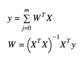
- Normal Equations (Closed-form Solution): Linear Regression can be solved in closed form.
In practice though, the matrix inversion can be quite difficult to calculate.
- No solutions: Linear Regression may not have a closed form/analytical solution due to non-invertible matrices
- Convex Problem: there is a guarantee of an optimum/minimum point that can be found
- The Best Fit Line minimizes the Mean Squared Error between the predicted and actual data points
- Gradient Descent/Stochastic Gradient Descent: this is often the preferred solver for large amounts of data.
- Correlation Factor: A perfect fit means correlation of 1.0 or -1.0. A lower absolute correlation value closer to 0.0 means lower predictability from input.
Closing Thoughts
Linear regression is not only the foundation and key building block of many complex machine learning algorithms, but also is extremely useful and effective in solving a lot of problems. These concepts can be as simple as a few lines of code, or as difficult as some complex statistical analysis that’s not covered here. We hope that we’ve covered enough material for you to apply this knowledge to your next project or give your memory lane a fresh restart.